2025 Devlog
🔗 June Links - Wolfire vs Steam, Indie vs AAA, What Does ‘Content Creator’ mean anyway?
2025-07-09I love when people catalog their interesting finds from around the web. IMO it’s a lot more pro-social than link aggregators or Bluesky or whatever.
It’s been a bit of a slow month for the newsletter since I’ve been busy programming, I’ll put up some new writing soon but in the mean time here are this month’s links. :)
Steam Stuff

If you have a game on Steam you probably got something like this in the mail and then panicked for a moment, before realizing that you’re not the one getting sued.
When I was a kid I used to hang out on macOS game development forums and try out other people’s games. I remember being particularly impressed by Black Shades, and even more so by Lugaru. Turns out the devs behind those games are still around–and they’re suing Valve:
- Wolfire’s complaint
- Wolfire’s blog post explaining the complaint
- “Valve’s 30% Platform Tax is Bad for Small Developers” (3rd party opinion)
Links unrelated to the lawsuit:
- Steamworks adds a sales data API
- Steamworks adds a new visual editor for events & announcements
- Chris Zukowski paid people to watch them browse Steam (old but good!)
Game Development

Indies like to trash talk AAA’s focus on physically based rendering, but I don’t think they remember how hard the less physically based lighting models were to work with. Acerola’s video on Persona 3 Reload is a great example of how modern rendering techniques are extremely useful, even for an extremely stylized game.
I don’t personally view AAA and indies as in competition, but to the extent that we are, rather than becoming Luddites we should instead form a deep understanding of what AAA is bad at, and then excel at exactly that.
The actual Luddites destroyed technology owned by their employers as a form of collective bargaining. I don’t really have any criticisms there. It’s just that if you’re an indie game developer, then by definition you are the employer, and you work on the most technical art form that exists right now, so you should probably embrace the technology right?
On a related note, it’s often possible to beat apparently best in class solutions even with limited time and resources by recognizing that others are trying to solve a more general form of the problem than is necessary to be useful. Maister’s fast game streaming video codec is a great example of this.
Other game development links…
- I uploaded my Zig SDL bindings
- Voronoi, Hashing and OSL
- Hash Functions for GPU Rendering
- I have a lot of this stuff implemented in GBMS
- Game Data comes to YouTube
- Efficient Gaussian blur with linear sampling
- Practical Gaussian filtering: Binomial filter and small sigma Gaussians
- Concentric Disk Sampling
- A Quick Overview of MSAA
- REAC 2025
Random Programming Thoughts

I’m starting to suspect that matklad is somehow spying on me, because he keeps writing blog posts that describe exactly how I think about programming.
If you’re using Zig on x64 Linux, consider pulling master–debug build times are getting fast. If you’re not using the build system yet, or you find it confusing, you should also check out Loris’s build system introduction video.
I have a little command line option parsing library I use in everything, but it’s kinda over-engineered and annoying to hack on. Here’s a much simpler way to parse options. I wonder if there’s a way to split the difference and still get a generated help menu?
Steve Klabnik is disappointed in the AI discourse. I am too.
Misc

The terms “influencer” and “content creator” always rubbed me the wrong way.
In some contexts, these labels make a lot of sense. It makes sense to call my list of influential people to send Steam keys to an influencer list.
It gets a bit wonky when you apply these labels to yourself though. Stealing an example, a musician wouldn’t call themselves a “merch seller” just because that’s how they pay the bills. Maybe YouTubers and Streamers aren’t “influencers”, but instead are entertainers, storytellers, documentarians, etc.
Hank Green and Ryg elaborate on these ideas here and here.
Other misc links:
- Please, critics, write about the filmmmaking
- Tukey
- The Shape of the Essay Field
- The Magnetic Shadow Effect
- This Graph Changed My Life
- Am I Cigarettes?
- Rory Sutherland - Are We Now Too Impatient to Be Intelligent?
Song of the Month
If you like the monthly links format, please steal it. Let’s bring some old internet energy back.
🔎 Antialiased Voronoi Diagrams
2025-06-10As part of my shader library, I’ve been playing with Voronoi Noise, and Voronoi Diagrams.
Voronoi noise is really fun, and surprisingly versatile.
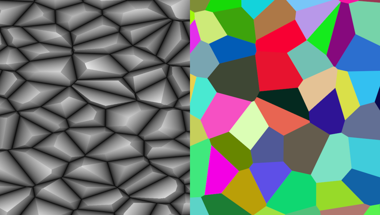
The gist of it is you divide your space into a grid, and then generate a random point for each grid cell. When you sample the noise, you get back the nearest of the random points. That’s it.
Here’s some glsl as an example:
#include <gbms/rand.glsl>
#include <gbms/hash.glsl>
#include <gbms/geom.glsl>
#include <gbms/constants.glsl>

struct Voronoi2 {
    // Position of the nearest point
    vec2 point;
    // ID of the nearest point (can has to pick colors/such)
    uint id;
    // Squared distance to the nearest point
    float dist2;
};

Voronoi2 voronoiNoise(vec2 p, vec2 period) {
    Voronoi2 result;
    result.dist2 = FLT_MAX;
    vec2 cell = floor(p);

    for (int x = -1; x <= 1; ++x) {
        for (int y = -1; y <= 1; ++y) {
            vec2 offset = vec2(x, y);
            uint id = pcgHash(floatBitsToInt(mod(cell + offset, period)));
            vec2 point = rand2(id) + offset;
            float dist2 = length2(point - fract(p));
            if (dist2 < result.dist2) {
                result.dist2 = dist2;
                result.point = floor(p) + point;
                result.id = id;
            }
        }
    }

    return result;
}
There’s a problem if you want to use this to draw colored cells though. There’s no antialiasing!
Not very pretty. How do we fix this?
We could just take multiple samples, and arguably that’s the most practical, but let’s see if we can solve it analytically.
In theory this would require us to to track all the points that influence our current fragment–up to 9 different points in 2D–but we can get away with just two. Anywhere that more than two points are influencing us is a corner, and we only care about antialiasing edges.
This is a pretty rote transformation of the previous code, but if you want to see it it’s here.
Once we have the nearest two points, we need to define a function that will calculate the blend factor between them. To do this, we can draw a line between the two points, and then check how close our sample is to the midpoint when projected onto that line. If it’s at the midpoint we have a 50% blend, and it falls off the further we get.
float voronoiAntialias(vec2 p, vec2[2] points, float grad) {
    vec2 line = normalize(points[1] - points[0]);
    vec2 midpoint = mix(points[0], points[1], 0.5);
    vec2 projected = points[0] + line * dot((p - points[0]), line);
    float dist_to_midpoint = length(projected - midpoint);
    return 1.0 - clamp(remap(0, grad, 0.5, 1, dist_to_midpoint), 0.5, 1);
}
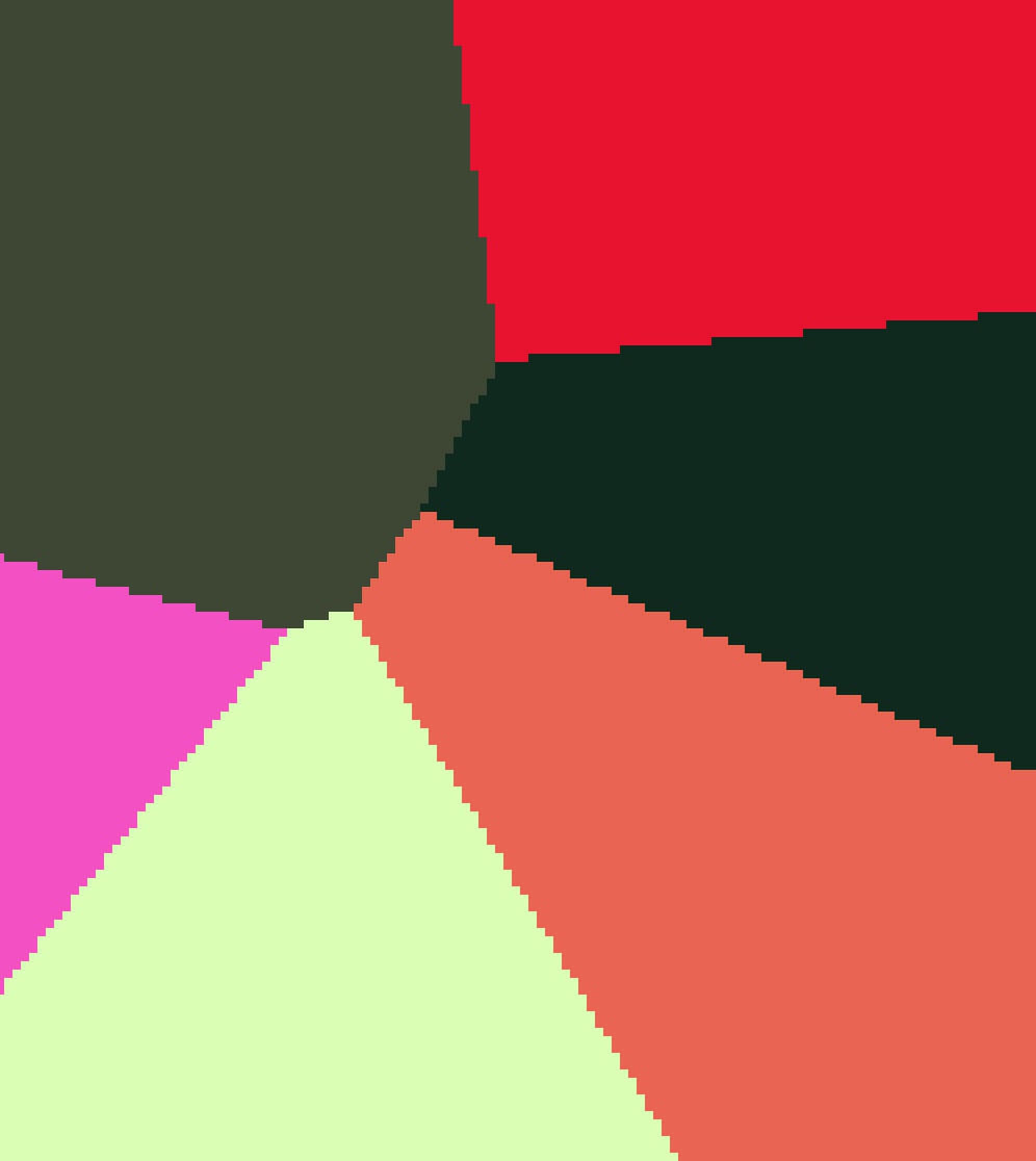
If we treat grad as an arbitrary threshold, we get a result like this:

As promised, we’re now blending the edges! We’ve set the threshold way too high though, and you can see artifacts in the corners as a result of only factoring in two points. Don’t worry, they won’t be visible once we fix the threshold.
If our image is always going to be rendered at a fixed size, then we can just set grad to the size of one pixel and get the results we want.
If our image might be moved around, rotated in 3D, stretched, etc, then we want to be a bit more flexible. Here’s what I use:
float voronoiGradient(vec2 p) {
    return compSum(fwidth(p)) / 4;
}
This isn’t technically correct–when the image is rotated by 45 degrees it’ll get sqrt(2) times more antialiasing–but it’s very convenient, and the artifacts aren’t visible in practice.
Here are the final results!


So, is this practical? I dunno, probably not. Most of the time you want to antialias at the end after you’ve done post processing on the noise. I also only derived it for 2D noise.
I have a specific effect in mind that needed the noise input to be antialiased, though, so it seemed worth deriving.
While I have you, here are some cool Voronoi patterns I created along the way because why not:


If this went over your head because you’re not experienced with noise, it’s not as complicated as you think, this just wasn’t written to be an intro to the topic.
Here are some great resources:
- The Book Of Shaders (intro level)
- inigo Quilezs’ Website (more advanced, but it’s inspiring stuff!)
- The Most Famous Algorithm In Compute Graphics (great explanation of Perlin noise)
Edit
I mentioned that taking more samples is the more practical approach, but not how to do it. Here’s how, imports are from gbms:
#include <gbms/noise.glsl>
#include <gbms/rand.glsl>
#include <gbms/aa.glsl>
#include <gbms/srgb.glsl>

// ...

// Generate one sample of Voronoi noise.
Voronoi2 center = voronoiNoise(texcoord);

// Estimate the size of a pixel. If you know you're rendering the
// surface straight on at a known resolution you can just put the
// exact value here instead.
float size = compSum(fwidth(texcoord)) / 2;

// Check if we're on an edge or not. I know everyone told you not to
// use branches in shaders, but they're wrong. The reality is more
// complicated and this type of thing really does work--profile it if
// you don't believe me.
if (abs(sqrt(center.dist2[0]) - sqrt(center.dist2[1])) < size) {
    // We're on an edge, get the constants for a 8x8 checkerboard
    // antialiasing kernel. We are throwing out the center sample
    // here, but I still found this pattern to be the fewest total
    // samples (8) that's indistinguishable from the analytic result.
    const uint samples = aa_checker4x4_samples;
    const vec2[samples] offsets = aa_checker4x4_offsets;
    const float[samples] weights = aa_checker4x4_weights;
    const float gain = aa_checker4x4_gain;

    // Sample the noise according to the kernel.
    vec3 antialiased = vec3(0);
    for (uint i = 0; i < samples; ++i) {
        Voronoi2 sample = voronoiNoise(texcoord + size * offsets[i]);
        antialiased += srgbToLinear(rand3(sample.id[0]) * weights[i]);
    }
    antialiased *= gain;
    out_color = vec4(antialiased, 1);
} else {
    // We're not on an edge, just display the single sample!
    out_color = vec4(srgbToLinear(rand3(center.id[0])), 1);
}
Left is the analytic solution, right is selective supersampling. I can’t tell the difference and we barely paid for it since we only did extra work on the edges.

Note that most images in this post were generated with the conversion from sRGB to linear incorrectly done after antialiasing instead of before. This has been corrected in the code samples, but the artifacts of this mistake are still visible in some of the images as slight “shadows” between cells!
🎂 May Links + Way of Rhea Anniversary Update
2025-05-29
I really like blogs & newsletters, and I really dislike social media.
The problem with blogs, though, is that they aren’t social. In an effort to combat this a little bit, I’m going to start sharing my favorite links at the end of every month.
If you enjoy the links, I recommend setting up an RSS reader and adding the authors to your feed. I use minflux, but there are lots of readers out there. Sites like YouTube also support RSS.
In unrelated news, this May marks the one year anniversary of Way of Rhea’s release!
To celebrate, the game is 50% off in the Cerebral Puzzle Showcase, and we just released the original sound track and a patch adding infinite mode.
Anyway, onto the links! I’m short on time today so I’m not going to editorialize, but I’ve sorted them by topic.
Blog Posts I Enjoyed
Game Programming
Game Design
Business
- Gaming’s Great Downsizing and the Garage-Band Game Economy
- Feral as a Moat
- How Empires Die
- Done with Twitter? You should start a blog instead
Technology
Other
- The haircutter
- Considering Democrats Blameless is a Medically Useless Diagnosis for the USA
- You’ll never be ready for anything that matters
- Why I Am Not A Conflict Theorist
- Two Toucans Canoe
- i beat impostor syndrome (and here’s how i did it)
- Every Bay Area House Party
- I Put a Toaster in the Dishwasher
Videos I Enjoyed

Game Programming
- The Most Famous Algorithm In Computer Graphics
- Your Colors Suck (it’s not your fault)
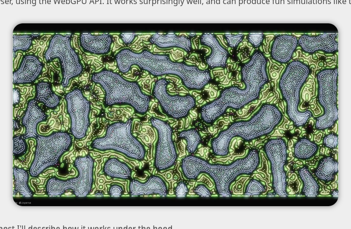
- I Tried Simulating The Entire Ocean
Business
- A good Xalavier Nelson Jr. interview with a clickbaity title
- How Successful Games Leverage Human Instinct
Technology
Games by Friends
Song of the Month
If you like the monthly links format, please steal it. Let’s bring some old internet energy back.
🕓 A More Objective Approach to Optimization
2025-04-22A couple of weeks ago while working on the beta release of my ECS, I noticed my command buffer abstraction was slow.
It turns out I was assuming the optimizer could do a few things it couldn’t. The fix wasn’t all that interesting, but it’s worth considering–how do you catch this sort of mistake?
For hot paths you could could manually check the generated code, but if you’re trying to analyze your entire program you’re going to want a profiler.

Alright, you’ve installed a profiler and instrumented your code–what next? It’s showing you a bunch of numbers, how do you assign meaning to them?
What counts as slow?
A reasonable but boring answer is that it’s context dependent. If you’re making a video game you might measure how many milliseconds the operation takes on your min spec hardware, and then compare that to your frame budget.
This is pragmatic, but it’s also subjective–how do you set the frame budget? How much time should you budget for physics? For rendering? How much headroom should you leave for the inevitable future gameplay features you haven’t thought of yet?
Answering the subjective question is it fast enough is part of the art of game development. However, there’s a more objective followup you should also be asking: How fast is it possible to go?
In theory this could be a very tough question to answer, but in practice it’s usually not. Here’s the answer for filling a command buffer:
@memcpy(cmdbuf, cmds);
You’re not gonna beat that. But you should probably try to tie it.
Comparisons to memcpy, ArrayList, and MultiArrayList are often very useful, because a lot of seemingly complex operations boil down to filling a buffer or buffers with data, and maybe doing some mild processing along the way.
If you can’t imagine how your operation could be thought of in these terms, you might want to double check that you really understand the work that’s being done.
Filling a command buffer is ultimately just copying bytes into an array, so we can determine our baseline by just copying the bytes of an example command buffer from one place to another. If we want to be slightly more fair, we can append the commands one at a time to an array list.
If you’re already tied with the baseline, great. Your work here is done.
What if it’s taking longer?
If the cause isn’t obvious, you can iteratively modify a copy of your algorithm–at the expense of correct results if needed–until the code is identical to the baseline.
At some point, one of these modifications is guaranteed to cause your operation to exhibit comparable performance to your baseline.
Congratulations, now you know both objectively how fast it’s possible to go, and what’s holding you back from achieving that performance!
Once you’ve maxed out this test it’s worth considering whether it’s possible to reasonably encode the same data in less bytes, but that’s a whole separate topic…
🧾 Fast Quaternion Normalization Proof
2025-03-02In my last post, I advocated for two different methods of accelerating inverse square roots when normalizing of quaternions:
- An approach for values very near to
1 - An approach for all other values
I was able to show empirically that method 1 converges for a reasonable range of inputs, but wasn’t able to prove it.
Matthew Lugg just sent me a proof that it converges for values between 0 and ~1.56!
In practice I switch to method 2 if I expect to need more than one iteration. Having a proof for the range of values it eventually converges for potentially allows for more precise trade offs, and at the very least gives me peace of mind that it’s correct within the range I’m using it.
My description of their proof follows.
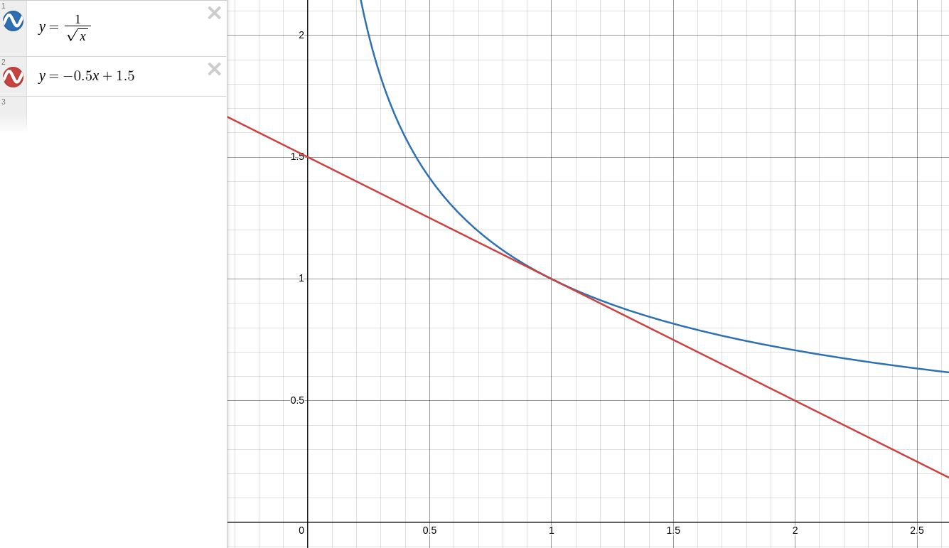
Consider the approximation:
1/sqrt(x) ~= -0.5x + 1.5
Using this to normalize a quaternion, you get:
q / sqrt(magSq(q))
If we substitute in our inverse square root approximation, we end up with the following equation:
q * (-0.5 * magSq(q) + 1.5)
Since all we’re interested in here is the magnitude, let’s rewrite this in terms of the magnitude. Take x to be the original magnitude, and y to be the approximately normalized magnitude:
y = |x * (-0.5x^2 + 1.5)|
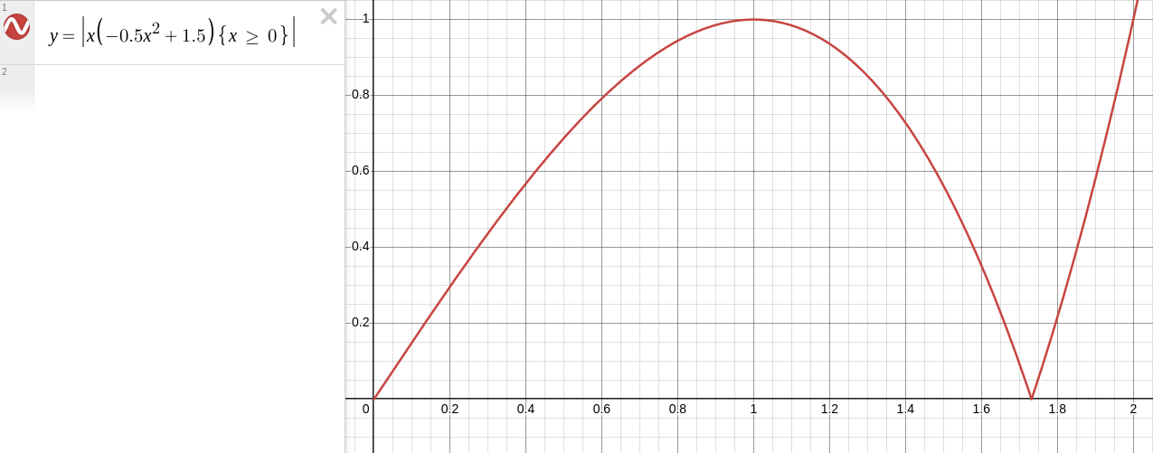
If we can show that within a given range out result y is always closer to 1 than our input x, then values in that range must converge.
We can do this by overlaying |y - 1| < |x - 1| on our graph. Anywhere this intersects with out curve, the approximation must converge:
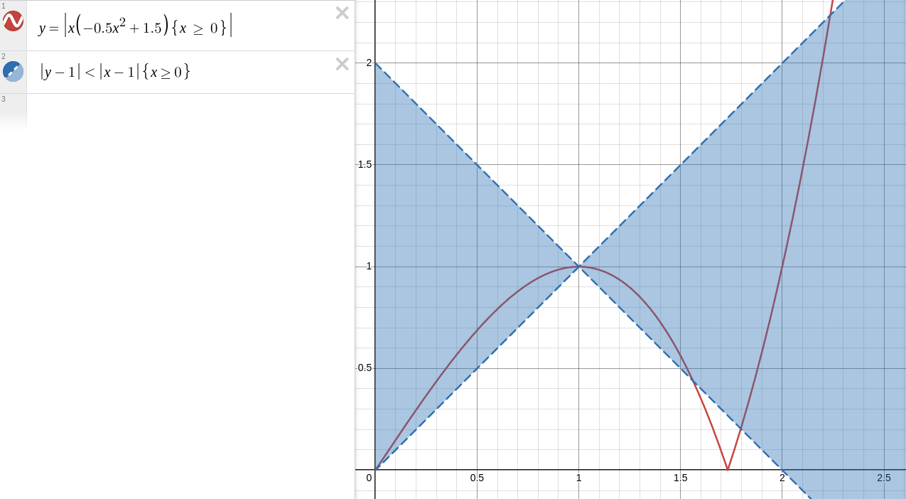
This is actually overly conservative, technically we could bounce further away before eventually converging–we’ll come back to this idea later.
The red line first crosses the blue area at 0, and then again at near 1.55. Let’s calculate the exact intersection:
# System of equations
y = 2 - x
y = |x * (-0.5x^2 + 1.5)|

# Substitute and simplify so we can solve for 0s
2 - x = |x * (-0.5x^2 + 1.5)|
0 = |x * (-0.5x^2 + 1.5)| - 2 + x
0 = |-0.5x * x^3 + 1.5x| - 2 + x

# Flatten the absolute value, discarding the second intersection
0 = -0.5x^3 + 2.5x - 2
Now we have a cubic equation. We can solve this ourselves, or throw it into a tool like Wolfram Alpha to get the intersection:
x = 0.5 * (sqrt(17) - 1) = 1.5615528128088303
So, our approximation must converge in the range (0, 1.5615528128088303)!
We could stop here, but my original claim was that this would converge until around ~2.24, which includes that suspicious area of the graph where the red line temporarily stops intersecting the blue area:
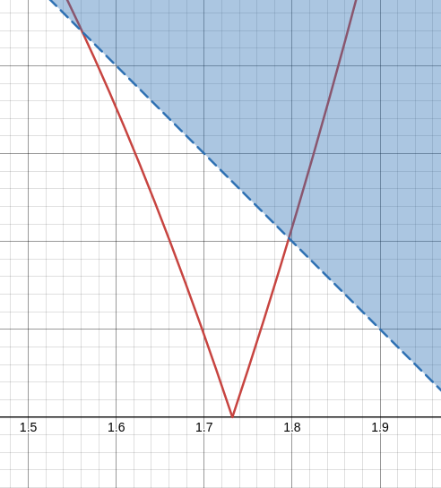
Remember when I said that checking for intersection with the blue area was overly conservative? It’s possible to get further from normal before eventually converging.
If you consider that all of the points in the problem area have y values of values between 0 and 1, it’s clear that any magnitudes in the problem area immediately yeet themselves out of the problem area into the left side of the plot, and therefore aren’t an issue.
…except the point that bounces off the x axis. At zero, our approximation outputs zero and gets stuck. So for this single point at exactly sqrt(3), it will fail to converge.
Do any other points eventually send us to sqrt(3)? If so, they’ll also diverge.
We don’t have to worry about points in the area we already proved converges since they always get closer to 1 and would have to get further from 1 to reach sqrt(3). However, this problem area might have more divergent points!
If we solve for where our approximation outputs sqrt(3), we get another divergent input. We can repeat this process iteratively to generate more divergent inputs:
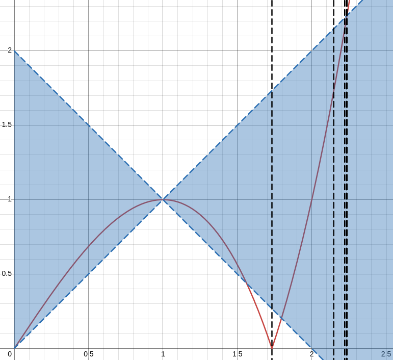
There appear to be an infinite number of these divergent inputs approaching sqrt(5). I was never going to catch this empirically, which is why it’s good to have proofs of this stuff.
It’s probably not possible to represent any of these precisely enough with 32 bit floats to trigger the issue, but now we have peace of mind that non shenanigans like this are waiting for us as long as we stay in that lower range.
In conclusion, the proposed approximation is proven valid for all magnitudes in the range (0, 1.5615528128088303), or more precisely, (0, 0.5 * (sqrt(17) - 1)), which is more than large enough for our purposes.
Outside of this range, you’ll start to have problems.
Thanks again to Matthew Lugg for figuring out this out and letting me share!
🔄 Fast Quaternion Normalization
2025-02-27Floating point division is slow, and square root is slower. What if I told you that you could approximate 1/sqrt(x) as y = -0.5x + 1.5?
Looks pretty bad right? Try zooming in.
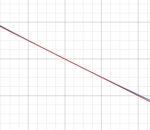
Hmm. Not so bad when you’re near x = 1.
If you’re using 1/sqrt(x) to normalize a quaternion after multiplication, this is likely all you need.
Multiplying two normalized quaternions by each other produces a third normalized quaternion with only a tiny bit of rounding error, so you’re always dealing with magnitudes near one. You just need to keep it from drifting so that your eventual rotation matrix doesn’t inadvertently scale your object.
This function isn’t magic–it’s just the tangent line of y = 1/sqrt(x) at x = 1. You can evaluate it in one instruction if your target supports fused multiply add:
/// Very fast approximate inverse square root that only produces usable
/// results when `f` is near 1.
pub fn invSqrtNearOne(f: anytype) @TypeOf(f) {
    return @mulAdd(@TypeOf(f), f, -0.5, 1.5);
}
(Side note–if this approximation is applied iteratively, the quaternion will approach normalcy if its initial magnitude is in the range Proof with corrected range is here!)(0, ~2.24), outside of that range it diverges. I verified this empirically but I’m not a good enough mathematician to prove it. If you manage to prove it let me know!
Alright, but what if you’re not near one? Maybe you lerped two quaternions together, or need a fast approximate inverse square root for some other purpose.
Turns out most CPUs have a hardware instruction for this now (e.g. on x86 it’s rsqrtss.) I’m not aware of any languages with platform independent intrinsics for this operation, but here’s a quick Zig snippet that will generate the instruction if your target supports it:
/// Fast approximate inverse square root using a dedicated hardware
/// instruction when available.
pub fn invSqrt(f: anytype) @TypeOf(f) {
    // If we're positive infinity, just return infinity
    if (std.math.isPositiveInf(f)) return f;

    // If we're NaN or negative infinity, return NaN
    if (std.math.isNan(f) or
        std.math.isNegativeInf(f) or
        f == 0.0)
    {
        return std.math.nan(f32);
    }

    // Now that we've ruled out values that would cause issues in
    // optimized float mode, enable it and calculate the inverse square
    // root. This generates a hardware instruction approximating the
    // inverse square root on platforms that have one, and is therefore
    // significantly faster.
    {
        @setFloatMode(.optimized);
        return 1.0 / @sqrt(f);
    }
}
This may also generate some extra instructions to refine the approximation. You could sidestep this if it’s undesired by writing per platform inline assembly, but it’s very fast regardless.
The above snippets are from my work in progress Zig geometry library for gamedev.
🧮 Fused Multiply Add
2025-02-22Quick performance tip. If you’re comfortable requiring support for FMA3 you should probably be using your language’s fused multiply add intrinsic where relevant.
For example, in Zig you’d replace a * b + c with @mulAdd(f32, a, b, c). This is much faster, and more precise.
This is an easy optimization, but the compiler can’t do it for you because replacing your arithmetic with more precise arithmetic isn’t standards compliant.
(Unless you’re using –ffast-math, then all bets are off WRT precision and you can just let the compiler do its thing.)
The only catch is, make sure you’re actually setting your target correctly! The compiler can’t ignore your request for muladd since that would change the precision of you result, so if you’re targeting a baseline CPU that doesn’t have it, you’ll end up emulating it in software and you’ll go slower instead of faster.
On desktop “big” core Intel & AMD CPUs have FMA since 2015, “small” core CPUs got it more recently.